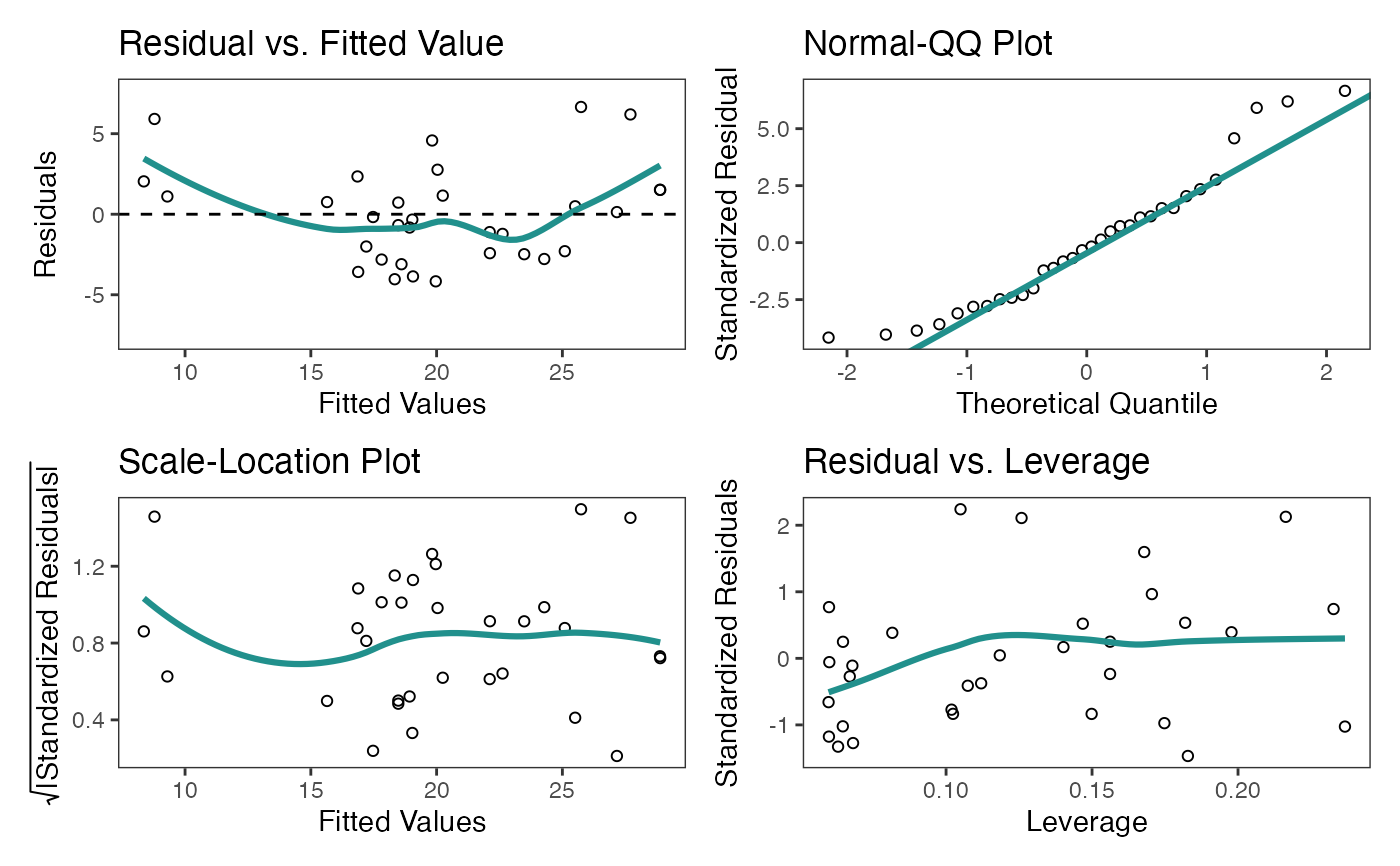
Regression Diagnostic Plots with ggplot2
Usage
gg_lm(
  model,
  which_plots = 1:4,
  cooksD_type = 1,
  standard_errors = FALSE,
  point_size = 1.5,
  theme_color = "#21908CFF",
  n_columns = 2
)
Arguments
- model
Model of class "lm" or "glm"
- which_plots
Choose which diagnostic plots to choose from.
Options are 1 = 'residual vs fitted', 2 = 'Normal-QQ', 3 = 'Scale-location', 4 = 'Residual vs Leverage', 5 = "Cook's Distance". 6 = "Collinearity". Default is 1:4- cooksD_type
An integer between 1 and 4 indicating the threshold to be computed for Cook's Distance plot. Default is 1. See details for threshold computation
- standard_errors
Display confidence interval around geom_smooth, FALSE by default
- point_size
Change size of points in plots
- theme_color
Change color of the geom_smooth line and text labels for the respective diagnostic plot
- n_columns
number of columns for grid layout. Default is 2
Details
Plot 5: "Cook's Distance": A data point having a large Cook's distance indicates that the data point
strongly influences the fitted values of the model. The default threshold used for detecting or classifying observations as outers is \(4/n\) (i.e cooksD_type=1)
where \(n\) is the number of observations. The thresholds computed are as follows:
cooksD_type = 1: 4/n
cooksD_type = 2: 4/(n-p-1)
cooksD_type = 3: 1/(n-p-1)
cooksD_type = 4: 3* mean(cook's distance values)
where \(n\) is the number of observations and \(p\) is the number of predictors.
Plot 6: "Collinearity": Conisders the variance inflation factor (VIF) for multicollinearity:
Tolerance = \(1 - R_j^2\), VIF = (1/Tolerance)
where \(R_j^2\) is the coefficient of determination of a regression of predictor \(j\) on all the other predictors.
A general rule of thumb is that VIFs exceeding 4 warrant further investigation, while VIFs exceeding 10 indicates a multicollinearity problem
References
Belsley, D. A., Kuh, E., and Welsch, R. E. (1980). Regression Diagnostics: Identifying Influential Data and Sources of Collinearity. New York: John Wiley & Sons.
Sheather, S. (2009). A modern approach to regression with R. Springer Science & Business Media.
Examples
model <- lm(mpg ~ wt + am + gear, data = mtcars)
gg_lm(model)